| ||||||||||||||||||||||||



https://twitter.com/mjgraves/status/1489291982262386697?s=21
https://twitter.com/samhlevey?s=21
Feb 2, 2022
Patricia and Christian talk to economics scholar, teacher and writer Sam Levey about real existing economic conditions (containing monopoly, monopsony, and oligopolistic price-setting power), the inadequate models used by economists to interpret these conditions, and a better way forward.
Please help sustain this podcast!
Patrons get early access to all episodes and patron-only episodes: https://www.patreon.com/MMTpodcast
For an intro to MMT:
Listen to our first three episodes: https://www.patreon.com/posts/41742417
All our episodes in chronological order: https://www.patreon.com/posts/43111643
All our episodes with Sam Levey: https://www.patreon.com/posts/43189679
Buffer Stocks: A Better Diagram, by Sam Levey: https://slevey087.medium.com/buffer-stocks-a-simpler-diagram-a462e9ea5359 ★
Monopoly Money: The State as a Price Setter by Pavlina R. Tcherneva:http://moslereconomics.com/wp-content/uploads/2018/04/Tcherneva_MonopolyMoney_2002.pdf
Monopoly Money Redux by Sam Levey: https://medium.com/@slevey087/monopoly-money-redux-a4d96f156f7
Our episodes laying out the MMT Job Guarantee:
Episode 4 - Fadhel Kaboub: What is the Job Guarantee?: https://www.patreon.com/posts/41742701
Episode 47 - Pavlina Tcherneva: Building Resilience - The Case For A Job Guarantee: https://www.patreon.com/posts/36034543
Modern Money and the War Treasury, by Sam Levey: http://www.global-isp.org/working-paper-no-123/
http://www.global-isp.org/wp-content/uploads/WP-123.pdf
2019
Our episodes about Modern Money and the War Treasury:
Episode 32 - Sam Levey: How Uncle Sam Paid For World War II (part 1): https://www.patreon.com/posts/30005574
Episode 33 - Sam Levey: How Uncle Sam Paid For World War II (part 2): https://www.patreon.com/posts/30112818
For information on their forthcoming MMT book, sign up to the Gower Initiative For Modern Money Studies mailing list: https://gimms.org.uk/
A list of MMT-informed campaigns and organisations worldwide:https://www.patreon.com/posts/47900757
Transcript for opening monologue: https://www.patreon.com/posts/61954919
We are working towards full transcripts, but in the meantime, closed captions for all episodes are available on our YouTube channel:https://www.youtube.com/channel/UCEp_nGVTuMfBun2wiG-c0Ew/videos
Show notes: https://www.patreon.com/posts/61954971
Buffer Stocks: A Simpler Diagram
A buffer stock is a price stabilization scheme. To run a buffer stock, some entity sets a target price of a particular good, and then buys and/or sells the good in whatever quantity is needed to move the market price to the target. The scheme operator thereby absorbs fluctuations in supply and demand, channeling them into changes in the size of the operator's inventory of the good — the "buffer stock" — rather than into changes in price.
Buffer stocks are a key concept for Modern Monetary Theory (MMT). In fact, so far as I know, using buffer stocks to organize a broader framing on macroeconomic policy is an original contribution of MMT that nobody else has put forward.
So it drives me nuts that the diagrams out there for explaining how buffer stocks work are so messy. Here's one example:

What I hope to do here is provide a simpler diagram for understanding buffer stocks. I'm not claiming revolutionary insights here — as we'll see below, this diagram is based on the common depiction of how central banks set interest rates. But hopefully you'll find it illuminating nonetheless.
Before we start though, a quick warning label: this diagram is a supply and demand diagram. I happen to believe that supply and demand diagrams, and the Perfect Competition model that lies behind most of them, are highly problematic ways to understand the economy and how prices are actually set. See here, here and here for some critique. This is especially true for some particular markets, eg. the labor market. In my view we must move beyond supply/demand in order to create satisfactory theories of distribution, inflation, etc. But that doesn't mean that it isn't a useful heuristic at times so long as the assumptions are made clear and a proper warning label is used, and this is one of those cases. So let's see it.
The basic model
In a buffer stock, the buffer stock operator stabilizes the price of a good within a range, by choosing a "sell price" and a "buy price" that form the top and bottom of that range. We'll start by assuming there's some standard downward-sloping demand curve out there. Above the buy price we will leave it be, but if the market price hits the buy price, then the scheme operator will jump in to buy whatever is necessary to keep the price from falling lower. Since these purchases contribute to demand, that gives us a combined demand curve that looks like this:

The downward sloping part comes from the market, representing the fact that the scheme operator does no buying if the market price is above its buy price, while the flat part is there because the buffer stock operator is willing to buy any quantity at the buy price.
Next we'll allow for some standard upward-sloping market supply curve, with the buffer stock operator jumping in to sell to prevent the price from rising above the sell price:

The upward sloping part comes from the rest of the market and represents that the scheme operator does no selling when the price is below the sell price, while the flat part of the curve is because the buffer stock operator is willing to sell any amount of the commodity to prevent the price from rising above their sell price.
The result when you combine them shows your buffer stock stabilized market with an equilibrium price and quantity.

In figure 4 here, it just so happens that the unassisted "market forces" are keeping the price in between the buffer stock buy and sell prices anyway, so the scheme operator doesn't actually have to do anything. But suppose that market demand falls a bit too much, i.e. the demand curve shifts to the left:
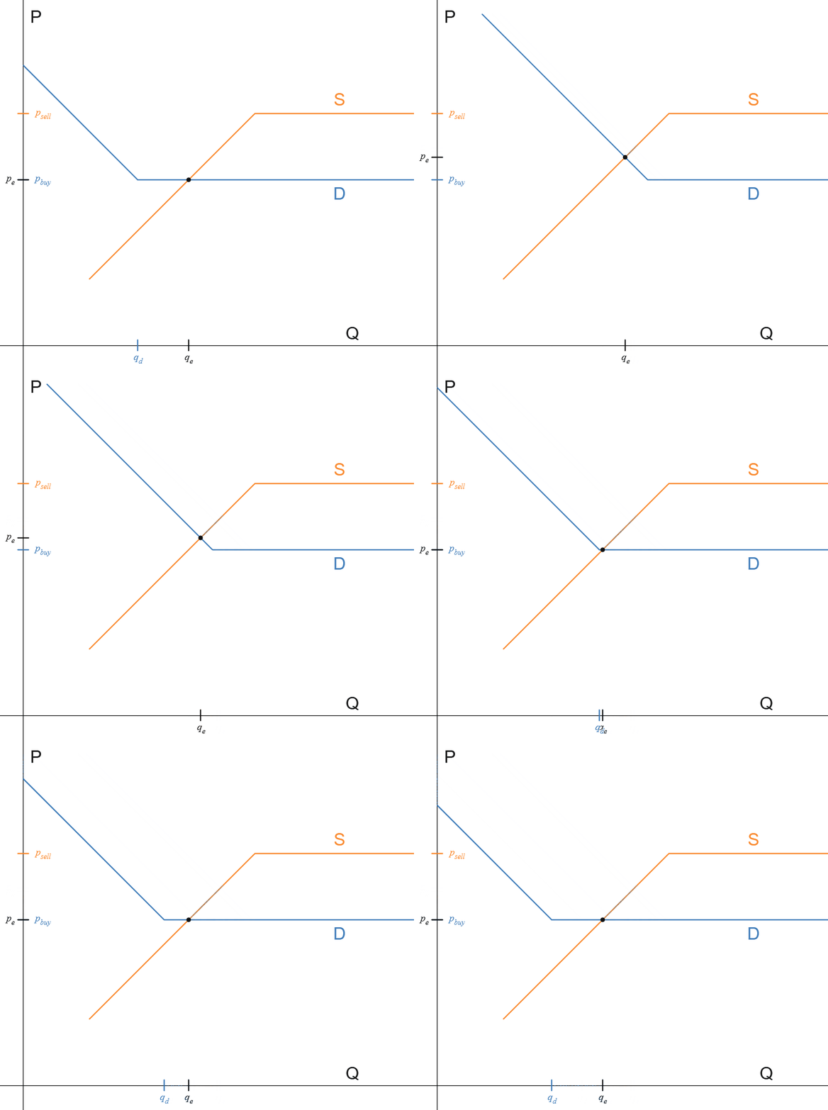
The equilibrium price has fallen but doesn't fall below the buy price, because the scheme operator jumps in. Notice that the scheme operator is buying the residual between what other suppliers want to sell at the buy price and what buyers want to buy at that price. This is shown as the gap between q_d and q_e. Of course, the scheme operator can only pull this off until they run out of money (or credit) to buy with.
If market supply had increased rather than demand decreased, the picture would have looked the same. But what if market supply falls, represented as the supply curve shifting to the left?
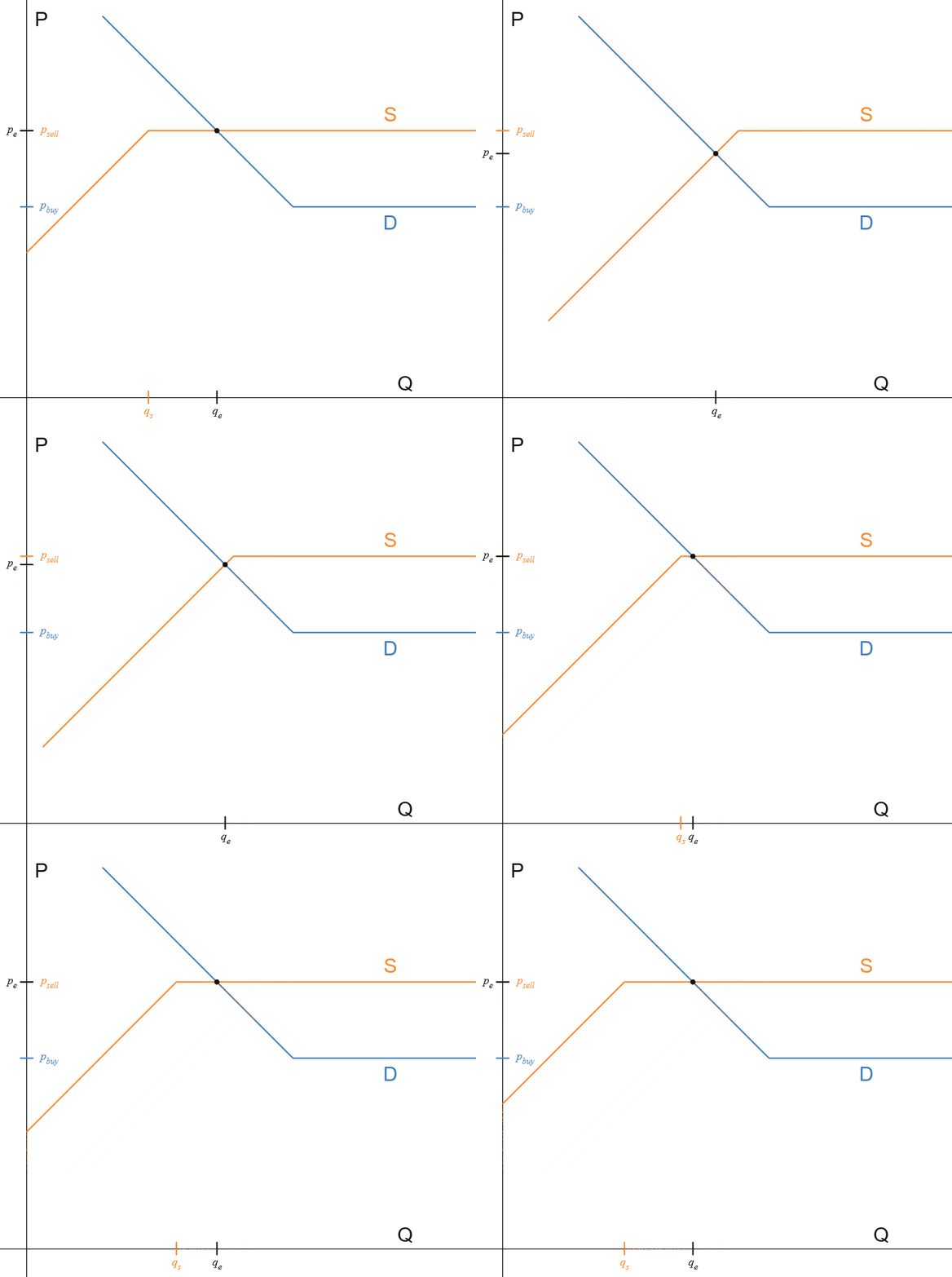
The price rises but doesn't rise past the sell price, because the scheme operator again jumps in, selling the residual between what the market is willing to supply at the sell price and what buyers want to buy at that price. This is shown as the gap between q_s and q_e. Of course, the scheme operator can only pull this off until they run out of inventory to sell.
Fiddling with prices
We could also ask questions about the relationship between the buy and sell prices. The gap between the buy and sell prices forms a 'corridor,' and the scheme operator can set this corridor as wide/narrow as they please, which would translate to looser/tighter control over the price. But what if they switched the prices, so that the buy price was higher than the sell price? Then things get dicey.

The curves don't intersect, so we don't have an equilibrium price or quantity…. what does this mean? Well, think about what other market participants might do if the buffer stock's buy price is above the sell price: I can make a risk-less profit by simply buying a unit of the good from the stock (at its sell price) and then selling that unit right back to the stock (at its buy price)! So how much am I going to want to buy? Infinity! I'll take every unit that the operator has, so I can sell them right back to the operator and pocket the difference between the buy and sell prices.
So, you can imagine that these two flat curves 'intersect at infinity.' Or, you might suppose that, because it takes inventories of money and the commodity to run this scheme, at some point off to the right the buffer stock runs out of one of these and the scheme becomes inoperable, so the curves stop being flat and resume their previous slopes, and therefore intersect.
Another interesting case: what if the buy and sell prices are set to the same price? Then, straightforwardly, the market price will exactly equal the buffer stock operator's single price. This is shown in figure 8 (whose flux capacitor vibe is an unintentional side benefit).

Figure 8 happens to show the special case that the market equilibrium price without the buffer stock transactions just so happens to equal the buffer stock price. In general this will not be true, as fluctuating market conditions prompt supply and demand curves to move, perhaps quite wildly. In general then we'd see cases that look more like figures 9 and 10. (See if you can work out for yourself what's going on in these pictures.)


Further comments
So that's the model. Before we go though I want to add some discussion that will paint a fuller picture.
What's a commodity anyway?
Above I was writing as if the scheme is always to stabilize the price of some commodity like grain or corn on one side, against money being used to buy it on the other. But of course it doesn't have to be this way. For one thing, the point might be more to stabilize the value of the money rather than the commodity — this is exactly how the gold standard worked, with the government buying and selling gold in order to lock the value of the currency to a particular amount of gold.
Or, we can imagine different items on each side: I guess hypothetically we could have barter markets with commodities on both sides…but more realistically, lots of real world buffer stocks have 'money,' or more generally financial assets, on both sides.
Consider a fixed exchange rate currency. To peg the local currency to a foreign currency, a central bank will run exactly the operations we've been discussing: buy your currency back (using foreign currency reserves) to keep its price from falling below the buy price, and sell your currency (buying foreign currency) to keep its price from rising above the sell price. As above though, the buy and sell price can form a corridor, or be set to the same price.
A case that actually fits the pattern of a "fixed-exchange rate currency" quite closely are bank deposits. The bank essentially runs a buffer stock to ensure that the value of their liabilities, the "deposits," are always exactly equal to the value of state money. That's why "$1" in your bank account is always exactly worth "$1" of paper money. The buy price and sell price are equal here, so we'd be using figures 8–10. (Note that the bank's ability to do this depends on it not running out of paper money, which is why we have the Fed and the FDIC as government backstops to make sure they don't.)
Whose operation is it anyway?
We've been tacitly assuming some sort of auction mechanism, which makes the idea of supply and demand curves, as well as a price that adjusts to equate supply and demand, a lot more plausible. However, it would really suck to be a buffer stock operator if you actually had to participate in an auction mechanism that forced you to specify a quantity rather than a price. That's because without knowing exactly what the market supply and demand are, you don't know what quantities would be needed to move the auction price to be within your corridor. You have to guess, and you'll probably guess wrong. The result is that the price probably would not stay within the corridor at all times.
What you'd like to do instead is remove yourself from that auction, and just post prices. That is, instead of guessing quantities that the market needs, let the market come to you. Any trader who encounters a price outside the buffer stock corridor can just decline that trade and come to the buffer stock instead. In that case then, there's really no reason for trades to ever happen outside of your corridor. (ALERT! The previous statement neglects all kinds of things like transaction costs, lack of liquidity, uncertainty, imperfect information, etc. But hopefully you get the idea.)
Central bank interest rate targets
If you follow monetary policy (skip this section if you don't), then you've probably seen a graph that looks like figure 11, depicting how a central bank can use a "corridor system" to hit its interest rate target in the inter-bank lending market:

This graph is of course the inspiration for the ones I showed above, so I'm not claiming to have had a wildly new thought. But that said, there are a few important differences between this graph and mine. While the 'price' on the vertical axis is the interest rate on inter-bank loans, the horizontal axis doesn't actually show the quantity of loans in that market. Instead it shows the amount of reserves that banks are willing to hold. Also, the market is decomposed in a different way: instead of showing borrowers and lenders separately, as you might if you drew the demand and supply of loans, the graph splits the world into the actions of commercial banks on the red line and the actions of the central bank on the blue line, so really the whole private market gets collapsed into the demand curve. (Coincidentally, I just read a recent explanation from Brian Albrecht about collapsing supply and demand curves into a single "total demand" curve, which is basically what's going on here.)
The upshot then is that the flat parts of these curves happen for different reasons. The flat part of the supply (blue) curve in Figure 11 is similar as above, it's because the buffer stock operator, the central bank, will add reserves in whatever quantity is needed to keep the interest rate within the corridor. But the the flat part of the demand (red) curve doesn't just show the actions of the buffer stock operator but actually involves the rest of the market too: it indicates that no bank would want to lend out reserves at a lower interest rate than it could get for just holding them (which is the Interest On Reserves (IOR) rate that the central bank pays). So, at any interest rate below that, banks would do zero lending in the inter-bank market, which is equivalent to saying they'd hold all the reserves that exist, whatever that amount might be.
The Job Guarantee and other one-way buffer stocks
Besides using buffer stocks as a descriptive model to make sense of existing institutions like fixed exchange rates and interest rate targets, MMT also applies the concept analogically for understanding the neoliberal approach to fighting inflation. Briefly, that strategy has been to use policy (primarily interest rate adjustments) to keep unemployment above a certain level (called the NAIRU, or Non-Accelerating Inflation Rate of Unemployment), on the basis that high unemployment would make it hard for workers to bargain for higher wages, which would then keep costs and therefore prices down. Because this method relies on an adjusting pool of unemployed people to stabilize prices, MMTers refer to this strategy as an unemployment buffer stock.
But we believe there is a better way here, and that's where MMTers go beyond using buffer stocks as descriptive, and start recommending that we add a major new buffer institution to the economy: a Job Guarantee (JG).
In a JG, the government would announce a fixed hourly wage, and then hire anybody who wants to work at this wage, to do small-scale local community service work. This is a buffer stock in labor, hence it also gets called an employment buffer stock (or labor standard, as a throwback to the gold standard). This too would stabilize the general price level by stabilizing wages —except it does so not by keeping wages down because people can't find jobs, but by channeling changes in market conditions into changes in the number of people the government hires, i.e. allowing the "stock" to float, at a fixed price. Stabilizing the price of basic labor should then feed through to price stability overall, both by stabilizing costs (as various prices and wages are set at a mark-up over basic labor) as well as demand (as the total demand for labor is always kept exactly at the full employment level). So the JG is meant to anchor the value of the currency in general (hence "labor standard").
You might notice though that this is only half of a buffer stock: the government only buys labor, it wouldn't sell labor. So, shouldn't that affect their ability to stabilize prices? The government could prevent the market price from falling below its buy price by buying the residual (as in figure 5 above), but how would they stop prices from rising if they can't sell the residual (as in figure 6)? In other words, what would happen if the number of workers employed in the JG fell toward zero? Would inflation start spiraling upward, and how would the government deal with this?
The answer is that they would have to use other aggregate demand (AD) management policies to bring the overall demand for labor back down to a level where at least some people are employed in the JG. (The minimum number of people that likely need to be in the JG for it to function properly at preventing inflation is called the NAIBER, or Non-Accelerating Inflation Buffer Employment Ratio). For simplicity, think about taxes: they could raise taxes, which would reduce incomes and therefore reduce private purchases of goods and services, which would reduce private demand for labor, so some workers would leave their private jobs and take up JG employment. (Of course, there are other sorts of policies besides taxes that could reduce demand for labor, such as cutting government spending, increasing private saving, shifting around imports and exports, increasing productivity, etc.)
But however it happens, how would it translate on our graph? Before we do that, this is another place where a warning label is in order: supply and demand graphs are a TERRIBLE way to understand the labor market. Basically, just don't do it! Again, I'm only doing it here to make a hand-wavey point that's not really specific to labor markets. If you want to talk about some labor-specific issue, like the minimum wage, just do not do it!
But anyway, since the government does not sell labor, the supply curve has no horizontal part, and the market looks like this:

If either the demand for labor were to increase (shift right) or the supply of labor were to fall (shift left), then the government would use taxes or other AD management tools to shift the non-JG part of the demand curve to the left, so that there's always a residual amount of labor for it to buy, keeping the market price at the buy price, which is the JG wage.
Conclusion
Buffer stocks aren't just a niche piece of agricultural economics; they are a powerful tool for understanding macroeconomics. And if we're going to place them so prominently in our explanation, we ought to have a clear, simple diagram that gives some intuition about how they work, so that's what I'm offering here. While there are dangers of indiscriminately throwing supply & demand graphs around, this buffer stock model is still useful for wrapping your head about things like bank deposits, fixed exchange rates, and the Job Guarantee.
バッファーストック:より単純な図。バッファー在庫は価格安定化です…| サム・リービー 2022年1月| 中くらい
バッファーストック:より単純な図
バッファーストックは価格安定化スキームです。バッファーストックを実行するために、一部のエンティティは特定の商品の目標価格を設定し、市場価格を目標に移動するために必要な数量で商品を購入および/または販売します。これにより、スキームオペレーターは需要と供給の変動を吸収し、価格の変化ではなく、オペレーターの商品在庫のサイズの変化、つまり「バッファーストック」にそれらを導きます。
バッファーストックは、現代貨幣理論(MMT)の重要な概念です。実際、私が知る限り、マクロ経済政策に関するより広範な枠組みを組織化するためにバッファーストックを使用することは、他の誰も提唱していないMMTの元々の貢献です。
ですから、バッファーストックがどのように機能するかを説明するための図が非常に乱雑であることに気づきます。これが1つの例です:
ここで私がしたいのは、バッファーストックを理解するためのより簡単な図を提供することです。ここでは革新的な洞察を主張していません。以下で説明するように、この図は中央銀行が金利を設定する方法の一般的な描写に基づいています。しかし、うまくいけば、それにもかかわらずあなたはそれが照らしているのを見つけるでしょう。
ただし、始める前に、簡単な警告ラベルを付けます。この図は需要と供給の図です。需要と供給の図、およびそれらのほとんどの背後にある完全競争モデルは、経済と実際の価格設定を理解するための非常に問題のある方法であると私は思います。いくつかの批評については、ここ、ここ、ここを参照してください。これは、特定の市場に特に当てはまります。労働市場。私の見解では、分配、インフレなどの満足のいく理論を作成するために、需要と供給を超えて移動する必要があります。しかし、それは、仮定が明確で適切である限り、それが時々有用なヒューリスティックではないという意味ではありません。警告ラベルが使用されており、これはその1つです。それでは、それを見てみましょう。
基本モデル
バッファーストックでは、バッファーストックオペレーターは、範囲の上限と下限を形成する「販売価格」と「購入価格」を選択することにより、範囲内の商品の価格を安定させます。まず、標準的な下向きの需要曲線があると仮定します。買い価格を上回ったままにしておきますが、市場価格が買い価格に達した場合、スキームオペレーターは価格が下がらないようにするために必要なものを何でも買いに飛び込みます。これらの購入は需要に寄与するため、次のような複合需要曲線が得られます。
下向きの傾斜部分は市場から来ており、市場価格が購入価格を上回っている場合はスキームオペレーターが購入を行わないのに対し、バッファーストックオペレーターは購入価格で任意の数量を購入する意思があるため平坦な部分があります。 。
次に、標準的な上昇傾向の市場供給曲線を考慮に入れます。バッファー在庫オペレーターが売りに飛び込んで、価格が売り価格を上回らないようにします。
上向きに傾斜している部分は他の市場から来ており、価格が売り価格を下回っている場合、スキームオペレーターは売りを行わないことを表します。一方、曲線の平坦な部分は、バッファーストックオペレーターが任意の金額を売りたいと考えているためです。価格が販売価格を上回らないようにするための商品。
それらを組み合わせた結果は、均衡価格と数量でバッファー在庫が安定した市場を示しています。
ここの図4では、支援されていない「市場の力」がとにかくバッファー株の売買価格の間に価格を維持しているため、スキームオペレーターは実際には何もする必要がありません。しかし、市場の需要が少し落ちすぎたとしましょう。つまり、需要曲線が左にシフトします。
均衡価格は下がっていますが、スキームオペレーターが飛び込んでいるため、購入価格を下回っていません。スキームオペレーターは、他のサプライヤーが購入価格で売りたいものと買い手が購入したいものの間の残差を購入していることに注意してください。価格。これは、q_dとq_eの間のギャップとして示されます。もちろん、スキームの運営者は、購入するお金(またはクレジット)がなくなるまでこれをやってのけることができます。
需要が減少するのではなく、市場の供給が増加した場合、状況は同じように見えたでしょう。しかし、供給曲線が左にシフトすることで表される市場供給が低下した場合はどうなるでしょうか。
価格は上昇しますが、売り価格を超えて上昇することはありません。スキームオペレーターが再び飛び込み、市場が売り価格で供給しようとしているものと買い手がその価格で買いたいものとの間の残差を売ります。これは、q_sとq_eの間のギャップとして示されます。もちろん、スキームのオペレーターは、販売する在庫がなくなるまでこれを実行することしかできません。
価格をいじる
また、売買価格の関係について質問することもできます。売買価格のギャップは「回廊」を形成し、スキームオペレーターはこの回廊を好きなだけ広く/狭く設定できます。これは価格のより緩い/より厳しい管理につながります。しかし、彼らが価格を切り替えて、買い価格が売り価格よりも高くなった場合はどうなるでしょうか。その後、物事は危険にさらされます。
曲線は交差しないので、均衡価格や数量はありません…。これは何を意味するのでしょうか?さて、バッファー株の買い価格が売り価格を上回っている場合、他の市場参加者がどうするか考えてみてください。株式から商品を(売り価格で)購入してから売るだけで、リスクのない利益を上げることができます。そのユニットは(購入価格で)在庫に戻ります!では、いくら購入したいですか?インフィニティ!オペレーターが持っているすべてのユニットを持っていくので、すぐにオペレーターに売り戻し、売買価格の差額をポケットに入れることができます。
したがって、これらの2つの平坦な曲線は「無限大で交差する」と想像できます。または、このスキームを実行するにはお金と商品の在庫が必要なため、右側のある時点でバッファーストックがこれらのいずれかを使い果たしてスキームが動作しなくなり、曲線が平坦でなくなり、以前の勾配を再開するため、交差します。
もう1つの興味深いケース:売買価格が同じ価格に設定されている場合はどうなりますか?そうすれば、簡単に言えば、市場価格はバッファーストックオペレーターの単一価格と正確に等しくなります。これを図8に示します(その磁束コンデンサの雰囲気は意図しない副次的な利点です)。
図8は、バッファー株取引がない場合の市場均衡価格がたまたまバッファー株価と等しくなるという特殊なケースを示しています。一般に、これは真実ではありません。変動する市況が需要と供給の曲線を、おそらく非常に激しく動かすように促すからです。一般に、図9および10のようなケースが見られます(これらの写真で何が起こっているかを自分で解決できるかどうかを確認してください)。
さらなるコメント
これがモデルです。行く前に、より完全な絵を描くいくつかの議論を追加したいと思います。
とにかく商品は何ですか?
上記では、穀物やトウモロコシなどの商品の価格を、もう一方の購入にお金が使われるのではなく、常に安定させるためのスキームであるかのように書いていました。しかしもちろん、このようにする必要はありません。一つには、商品よりも金の価値を安定させることが重要かもしれません。これはまさに金本位制の仕組みであり、政府は通貨の価値を特定の金額に固定するために金を売買します。金の。
または、それぞれの側で異なるアイテムを想像することができます。仮想的には、両側に商品がある物々交換市場があると思います…しかし、より現実的には、多くの現実世界のバッファー株は、両側に「お金」、またはより一般的には金融資産を持っています。
固定為替レートの通貨を考えてみましょう。現地通貨を外貨にペグするために、中央銀行は私たちが議論してきた操作を正確に実行します:価格が購入価格を下回らないように(外貨準備金を使用して)通貨を買い戻し、通貨を売ります(外貨の購入)、その価格が販売価格を上回らないようにします。ただし、上記のように、売買価格はコリドーを形成することも、同じ価格に設定することもできます。
「固定相場制通貨」のパターンに実際によく当てはまるのは銀行預金です。銀行は基本的に、負債の価値である「預金」が常に国のお金の価値と正確に等しくなるように、バッファーストックを実行します。そのため、銀行口座の「$ 1」は、常に「$ 1」の紙幣の価値があります。ここでは、買い価格と売り価格が等しいため、8〜10の数字を使用します。(これを行う銀行の能力は、紙幣が不足していないことに依存していることに注意してください。そのため、FRBとFDICは、政府がそうしないようにするためのバックストップとして使用しています。)
とにかく誰の操作ですか?
私たちは、ある種のオークションメカニズムを暗黙のうちに想定してきました。これにより、需要と供給の曲線のアイデアと、需要と供給を等しくするように調整される価格がはるかに妥当になります。ただし、実際にオークションメカニズムに参加して、価格ではなく数量を指定する必要がある場合は、バッファストックオペレーターになるのは非常に困難です。これは、市場の需要と供給が正確にわからないと、オークション価格を廊下内に移動するために必要な数量がわからないためです。あなたは推測しなければなりません、そしてあなたはおそらく間違って推測するでしょう。その結果、価格はおそらく常に廊下に留まらないでしょう。
代わりにやりたいのは、そのオークションから自分を削除し、価格を投稿することです。つまり、市場が必要とする量を推測する代わりに、市場があなたのところに来るようにします。バッファーストックコリドー外の価格に遭遇したトレーダーは、そのトレードを拒否して、代わりにバッファーストックに来ることができます。その場合、あなたの廊下の外で取引が行われる理由は実際にはありません。(警告!前のステートメントは、取引コスト、流動性の欠如、不確実性、不完全な情報などのすべての種類のものを無視しています。しかし、うまくいけば、あなたはアイデアを得るでしょう。)
中央銀行の金利目標
金融政策に従っている場合(そうでない場合はこのセクションをスキップしてください)、中央銀行が「回廊システム」を使用して金利目標を達成する方法を示す図11のようなグラフを見たことがあるでしょう。銀行間貸付市場:
もちろん、このグラフは私が上に示したもののインスピレーションであるため、私は非常に新しい考えを持っていたとは主張していません。とはいえ、このグラフと私のグラフにはいくつかの重要な違いがあります。縦軸の「価格」は銀行間ローンの金利ですが、横軸は実際にはその市場のローンの量を示していません。代わりに、銀行が保有する用意がある準備金の量を示します。また、市場は別の方法で分解されます。ローンの需要と供給を描いた場合のように、借り手と貸し手を別々に表示する代わりに、グラフは世界を赤い線の商業銀行の行動と行動に分割します青い線の中央銀行の、それで実際に全体の民間市場は需要曲線に崩壊します。(偶然にも、私はちょうど読んだ需要と供給の曲線を単一の「総需要」曲線に折りたたむことについてのBrianAlbrechtからの最近の説明。これは、基本的にここで起こっていることです。)
結果として、これらの曲線の平坦な部分はさまざまな理由で発生します。図11の供給(青)曲線の平坦な部分は上記と同様です。これは、中央銀行であるバッファーストックオペレーターが、廊下内の金利を維持するために必要な量の準備金を追加するためです。しかし、需要(赤)曲線の平坦な部分は、バッファーストックオペレーターの行動を示しているだけでなく、実際には市場の他の部分も含んでいます。これは、低金利で準備金を貸し出したい銀行がないことを示しています。それらを保持するだけで得られるよりも(中央銀行が支払う利息(IOR)レート)。したがって、それより低い金利では、銀行は銀行間市場でゼロ貸付を行います。これは、存在するすべての準備金を保有すると言うのと同じです。
仕事の保証および他の一方向の緩衝株
MMTは、固定相場制や金利目標などの既存の制度を理解するための記述モデルとしてバッファーストックを使用するだけでなく、インフレと戦うためのネオリベラルなアプローチを理解するためにこの概念を類推的に適用します。簡単に言えば、その戦略は、高い失業率は労働者がより高い賃金のための掘り出し物、それはそれからコストを保ち、そしてそれ故に価格を下げるでしょう。この方法は、価格を安定させるために失業者のプールを調整することに依存しているため、MMTerはこの戦略を失業バッファー在庫と呼びます。
しかし、ここにはもっと良い方法があると信じており、MMTerはバッファーストックを記述として使用するだけでなく、経済に主要な新しいバッファー機関であるJob Guarantee(JG)を追加することを推奨し始めています。
JGでは、政府は固定時給を発表し、この賃金で働きたい人を雇って、小規模な地域社会奉仕活動を行います。これは労働の緩衝在庫であるため、雇用緩衝在庫(または労働基準)とも呼ばれます。、ゴールドスタンダードへの逆戻りとして)。これもまた、賃金を安定させることによって一般的な価格水準を安定させるでしょう。ただし、人々が仕事を見つけることができないために賃金を抑えるのではなく、市況の変化を政府が雇用する人々の数の変化に向けることによって、つまり、固定価格でフロートする「ストック」。基礎労働の価格を安定させることは、コスト(さまざまな価格と賃金が基礎労働よりも値上げされるため)と需要(労働の総需要が常に維持されるため)の両方によって、全体的な価格安定につながるはずです。完全雇用レベルで)。したがって、JGは、一般的な通貨の価値を固定することを目的としています(したがって「労働基準」)。
お気づきかもしれませんが、これはバッファーストックの半分にすぎません。政府は労働力を購入するだけで、労働力を販売することはありません。それで、それは価格を安定させる彼らの能力に影響を与えるべきではありませんか?政府は、残差を購入することで市場価格が購入価格を下回るのを防ぐことができますが(上記の図5のように)、残差を販売できない場合(図6のように)、価格の上昇をどのように阻止しますか?言い換えれば、JGで雇用されている労働者の数がゼロに向かって減少した場合はどうなるでしょうか。インフレは上向きにスパイラルし始めますか、そして政府はこれにどのように対処しますか?
答えは、労働需要全体をJGで少なくとも何人かの人々が雇用されているレベルに戻すために、他の総需要(AD)管理ポリシーを使用する必要があるということです。(インフレを防ぐためにJGが適切に機能するために、JGにいる必要があると思われる最小人数は、NAIBER、または非加速インフレバッファー雇用率と呼ばれます。)。簡単にするために、税金について考えてみてください。税金を引き上げると、収入が減り、商品やサービスの個人的な購入が減り、民間の労働需要が減ります。そのため、一部の労働者は、個人の仕事を辞めてJGの雇用に就きます。(もちろん、税金以外にも、政府支出の削減、個人貯蓄の増加、輸出入のシフト、生産性の向上など、労働需要を減らす可能性のある他の種類の政策があります。)
しかし、それがどのように起こったとしても、それは私たちのグラフでどのように変換されますか?その前に、これは警告ラベルが必要なもう1つの場所です。需要と供給のグラフは、労働市場を理解するためのひどい方法です。基本的に、それをしないでください!繰り返しになりますが、私はここでそれを行っているのは、労働市場に実際には固有ではない、手を振るようなポイントを作るためだけです。最低賃金のような労働特有の問題について話したいのなら、それをしないでください!
しかし、とにかく、政府は労働力を売っていないので、供給曲線には水平部分がなく、市場は次のようになります。
労働需要が増加する(右シフト)か、労働供給が減少する(左シフト)場合、政府は税金またはその他のAD管理ツールを使用して、需要曲線の非JG部分を残されたので、市場価格をJG賃金である購入価格に保ちながら、購入するための残余労働量が常に存在します。
結論
バッファーストックは、農業経済学のニッチな部分ではありません。それらはマクロ経済学を理解するための強力なツールです。そして、それらを説明の中で非常に目立つように配置する場合は、それらがどのように機能するかについての直感を与える明確で単純な図を用意する必要があります。それが私がここで提供しているものです。需要と供給のグラフを無差別に投げかける危険性はありますが、このバッファー在庫モデルは、銀行預金、固定為替レート、ジョブ保証などについて頭を悩ませるのに役立ちます。

0 件のコメント:
コメントを投稿